Optical Flow Sensors

Exploring the capabilities of optical flow sensors by transforming an old optical mouse into a handheld motion tracking device.

If you’re interested in the field of robotics and computer vision systems, you’ve likely heard of optic flow sensors. But what exactly are they, and how are they used today? In this article, we’ll take a closer look at the concept of optic flow and explore an old project that recycles one into a handy measuring tool.

What is Optical Flow?

Optical flow is foremost a human phenomenon, and it refers to our visual perception of motion, caused by either the movement of the observer or the motion of the objects in our environment.

To put this into context, see if you can recall sitting on a train gazing out of the window, and picture the scenery rushing past your eyes. You may not realize it but at the time your brain was playing a real-time game of “spot the difference” in the consecutive images its sees, unconsciously analyzing the movement of shapes, colours and textures as they traverse your field of view.

We build a kind of 2D matrix of visual cues that inform our brain of the direction and magnitude of movement in parts of our vision (this is the raw optic flow data). We then effortlessly process this raw data to interpret information like how fast and in which direction the objects we see are moving.

Why is this useful?

We can use this optical flow data to separate parts of a 2D image in 3D space. Consider in the train example, how objects near the observer will move faster across an image than ones in the background. This uneven distribution of optic flow is known as motion parallax. Regions of similar motion are grouped together to segment the image into different areas or objects. This process helps us acquire a sense of depth in what we see, and even with one eye shut we can still navigate and avoid obstacles in 3D space despite having most of our depth perception from Stereo-Vision (comparing images from the left and right eye).

For humans, Optical Flow forms a key piece of visual sensorial information that when combined with other signals from the vestibular system (fluid in the inner ear), auditory (sound) and proprioceptive inputs (knowing where your limbs are) all combined by the brain, guide actions such as walking, reaching, and avoiding obstacles (aka human locomotion) – pretty nifty.

Optical flow in computer vision

If we replace the human eye with a camera sensor, we can in theory emulate biological optical flow by analyzing a sequence of images (aka video). Techniques pioneered by Horn–Schunck in the late 1980s (link) are still in use today and modern derivates like Lucas-Kanade and Farneback, are used heavily in machine vision tasks like video compression and stabilization. And we can even use that handy parallax depth information to build accurate 3D models of an environment with just one camera in a process called structure from motion. So how do these techniques work?

The main challenge in estimating optical flow is trying to match corresponding pixels to the same objects in subsequent images. The starting point used by Horn–Schunck was a “brightness consistency assumption” that is, if two images are taken in quick succession, we can probably assume that not much has changed in the scene.

Therefore pixel intensities are mostly translated from one frame to the next. In reality, this method has some major limitations, for example, changes in global illumination, shadows or surface reflections will all break those basic assumptions. However, if we can keep the time difference between subsequent images low (high FPS) and global illumination consistent this method works quite well in practice.

To illustrate this concept, have a look at the two images below. These are 8×8 grayscale frames, the first taken at time t=1 and the second an (arbitrarily) small amount of time later at t=2.

As a starting point let’s choose the brightest pixel in the first image, we see that a pixel with an intensity of 255 is located at (x =3, y=3). In the next image, we find a similar pixel with the same intensity is now located at (x=5, y=4).

Therefore, we can assume this object has moved 2 pixels right and 1 down. With this information, we can plot the velocity and direction of motion for that pixel. All we need to do is repeat this process taking into account all the remaining intensities in the image and we can develop a rough 2D velocity field representing optical flow, illustrated above by a series of arrows. In reality, the optical flow equation is a tad more complicated to solve mathematically. As methods here rely on a Taylor Series approximation of an image that results in equations with two unknown variables, this is known as the Aperture Problem.

The Aperture Problem

The problem can be understood visually if you look at this image, here the grating appears to be moving both down and to the right, perpendicular to the orientation of the bars. But if you look more closely it is also true that the stripe could be moving in other directions, such as only down or only to the right. It is impossible to determine unless the ends of the bars become visible in the aperture.

To solve this problem, all-optical flow methods introduce additional constraints and assumptions for estimating the actual flow, if you want to learn more about these methods (I definitely don’t understand them all), I found this a useful source of information link.

Live demo with your camera 📸

(This demo runs entirely on your device, no images are sent or stored.)

Enough theory, let’s demonstrate a live optical flow estimation on your device. Here is demo written in P5.js that is computing a real-time optical flow estimation on your camera feed.

The demo works best if you place your phone down somewhere still and then move around in the scene.

The length and colour of the arrows relate to the velocity component of the optical flow field. The optic flow code is based on some opensource code by “Anvaka” on GitHub, If you would like to have a look at the code see below for the link.

Balls! The origins of the optical flow sensor

Outside of a few niche applications, Horn and Schunk’s work on optical flow algorithms initially failed to find a place in mainstream products. That was until it was widely adopted in the design of a new and improved optical computer mouse.

In the early days of personal computers, mice originally used weighted balls that rolled around encoder wheels, this was an expensive and unreliable solution due to the buildup of dirt. At the time these mice were so troublesome that the biggest computer manufacturer IBM, even released a tongue-in-cheek memo about the notorious “mouse balls” stating that;

“Each person should have a pair of spare balls for maintaining optimum customer satisfaction… and any customer without properly working balls is an unhappy customer.” Source

The need for a more robust solution eventually led Stephen B. Jackson to patent the first optical mouse design in 1988 for XEROX. The mouse featured a small light source, lens, and camera chip. As it had no moving parts, it became widely accepted as a more reliable and cost-effective solution. With the decrease in the cost of computing power, it became possible to embed image-processing chips right into the mouse, allowing optical flow calculations to be performed on the device itself.

Today, modern mice still retain the fundamental design principles of Jackson’s first optical mouse with several of the key features optimized specifically for optical flow calculation.

The sensors in modern optical mice run at high frame rates (Gaming mice can clock in over 10,000 FPS) to ensure the seamless translation of pixel intensities from one frame to the next. A controlled internal light source, such as an LED, is used to maintain Horn and Schunk’s brightness consistency assumption between frames and reduce the impact of changes in external illumination. The light source is cleverly directed at the surface at a shallow angle to enhance contrast in surface texture, producing an ideal image for optical flow analysis. This same principle is also seen in Dyson’s dust-hunting vacuum cleaners with frikin’ lasers.

Optic flow sensors used outside of computer mice?

Despite being primarily designed for computer mice, I have noticed them appear in a number of applications beyond pushing a cursor around your screen.

If you look inside a Nest Thermostat, you’ll notice there isn’t a rotary encoder or potentiometer in sight to detect the rotation of its outer ring. Rather than conventional sensing methods, the thermostat uses an optical flow sensor called an ADBM-A350 from Avago.

The ADBM-A350, which is marketed as a “Finger Sensor,” is a more familiar component than you would first think. A little digging though the datasheet reveals a package that is instantly recognisable as the almighty trackpad once used on millions of Blackberry mobile phones. In the Nest thermostat rather than looking for a finger, this sensor works by observing the inside of the brushed aluminium dial providing precise position feedback as it turns.

It’s interesting to note that similar to computer mice early Blackberry models started with a rolling trackball design before transitioning to optical flow sensing.

Why did Nest choose an optical flow sensor?

Non-contact - Great for User Experience

To justify its premium pricing, it is essential that the user experience and haptic feedback of the product’s main touchpoint (the big dial rotation) feels equally premium. Engineering the smoothness of rotation is much easier without physical connections to encoders, eliminating the sensation of gear teeth meshing and cyclical torques from misaligned gears. (I’m looking at you Amazon Alexa – link)

Lower Component Count

Optical sensors also allow for the use of existing parts of the device’s casework to track movement, whereas alternatives like magnetic and optical encoders always require an additional encoded surface for movement detection (a magnetic strip with alternating poles or a printed optical surface are common).

A missed opportunity? Why did Nest not use the optical flow sensor for button detection?

Pressing the dial into the product, allows a user to select an option from the on-screen menus, this action moves the entire ring assembly along the rotational axis. This motion is ultimately limited by a small dome switch on the PCB that detects the user’s input. To me at least, the haptics of this “click” feel mushy and underwhelming as they are driven by the snap of a rather cheap dome switch.

Considering that the product already has an optical sensor that is perfectly capable of detecting both the “in and out” movement (in the X direction) the ring as well its rotation (in the Y direction), perhaps the designers could have engineered a more satisfying feeling haptic for the “click” with some nice detents and used the optic flow sensor for the “button” detection instead of relying on a dome switch. Just a thought…

Proof of Concept...

A handheld measuring tool made with an optical flow sensor from an old mouse

Despite being more expensive than some traditional sensors that measure and track movement, I think optical flow sensors can offer several unique benefits and unfortunately are often overlooked.

I used an optical flow sensor in a university project back in 2017 and built a device that repurposed an old optical mouse into a digital distance-measuring tool. The device was controlled by an Arduino, had simple buttons and a screen that could be used to take real-world measurements just by sliding it across a surface.

The project was essentially a proof of concept that seemed to work quite well and was surprisingly accurate. If you are interested I have outlined some details about the electronics, software and mechanical design in the following section.

Credit to Tom Murton , Tak Chi-Ho and Michelle Okyere for supporting this work back in 2017!

1. Electronics & Hardware

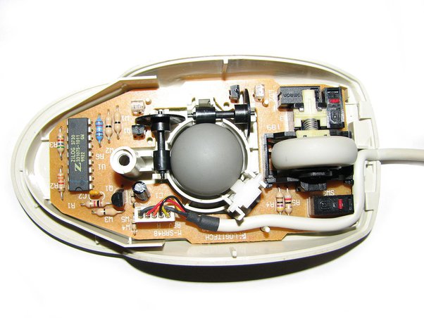
The first step is to gain access to the optic flow sensor inside the mouse. Removing a single screw separates the plastic casework and reveals a single-sided PCB, highly cost-optimized with only a few components. The optic flow sensor is a Logitech 361335-a000 that handles all the image processing from a 16×16 pixel image sensor in the center of the PCB.

After a bit of digging, it turns out that the simplest way of accessing the navigation data sent by the Logitech IC is to connect an Arduino to the PS2 connector on the PCB, and decode the serial data that the mouse would normally send to a computer. The PS/2 protocol was widely used in the 1990s and early 2000s, but has since been replaced by USB (Universal Serial Bus) communication in most computer peripherals. The connector uses 4 pins that we must hook the Arduino up to: Clock, Data, Ground and 5V.

Label	Component	Function
A	Microswitches (x3)	Left/Right/middle mouse click buttons.
B	Light Gate (Double Slit)	An IR LED and dual photodiode creates a simple light gate for the optical encoder on the mouse wheel to enable the scroll function.
C	Optical Sensor IC	This IC Captures a 16x16 pixel image of the surface and sends the data to the main IC for processing.
D	Connector	This connector terminates the PS2 cable on the PCB and provides a good entry point to monitor data without modifying the circuit board.
E	Illumination LED	A red LED illuminates the region under the optical sensor at a shallow angle, to maximize contrast by casting shadows to emphasize the surface roughness for optical tracking.
F	Logitech 361335-a000 IC	This is a custom IC that handles image processing and the PS2 communications.

Casework Design - Repackaging recycled components

Most of the original plastic components from the mouse were not usable in the final design and only the PCB, lens, and two microswitches were kept.

To make the device work independently from a computer, a number of additional components were added and housed in a new 3D Printed casework.

This included 2 AA batteries that could power the device through a 5V boost converter. An OLED screen would read out the final measurements and a piezo buzzer and LED were also included to indicate when a measurement was being taken.

The accurate positioning of the recycled optical components, specifically the lens and image sensor, relative to the tracking surface was crucial. Therefore the relevant features in the original moldings were carefully measured and reproduced in a new component I call the “Lower Platform” that accurately locates the lens and optical sensor.

A second 3D print called the”Upper Platform” was designed to accommodate the remaining components above the PCB.

The stack was then enclosed by an “Outer Casework” that has mounting bosses to secure the OLED Screen and the 2 micro switches.

Casework Design - Fastenings

Plastic thread-forming screws from TR Fastenings were used to secure all the components in the design instead of embedding nuts or thread inserts.

A note on Self Tapping Screws for plastics – Using standard self-tapping screws in plastic parts can cause a number of headaches. For example the plastic material is liable to burst due to stresses that build up in the assembly. Inserting the screws into metal inserts overcomes the problem but adds to the procurement and assembly costs.

These screws, also known as “Thread-forming Screws,” have sharper threads than self-tapping screws and are specifically designed for plastic housings. They are affordable and simple to use as long as you follow the manufacturer’s guidelines on boss dimensions. There are a range of thread angles depending on the hardness of the material you are fastening. For this build a thread angle of 60 degrees was ideal for the softer SLS Nylon that we 3D printed the casework in.

TR fastenings, Plas-Fix® Screws Link – ACCU also have equivalent Polyfix Screws – Link

Casework Design - Cantilever Button

The reused microswitches from the mouse provide a means for the user to start and stop measurements. To activate these switches, a cantilever section was added to the outer casing. The casework only needs to displace the switch by 0.6mm to activate it.

To recreate the feel of the original mouse click, I measured the force required to activate the original click at 73.5g. By treating the casework as a simple cantilever beam and using a bit of math, the necessary geometry can be calculated to replicate this force.

The cantilever beam, which is used to actuate the microswitches is governed by the equation for deflection (δmax). This equation considers the force required (P), the Young’s modulus (E) of the material, the second moment of area (I) of the beam, and its length (L).

As the beam is a rectangular cross-section and designed to be 10mm wide and 1.2mm thick the second moment of the area can be calculated first. Plugging this and the required deflection (set at 0.6mm), force (measured at 73.5g) and Young’s modulus for the SLS Nylon (2.3GPa) calculates a beam length of around 43.3mm.

Here you can see that the cantilever buttons modelled into the casework above the 2 micro-switches.

2. Software

Navigation data decoding

The mouse transmits navigation data to the host computer via the PS/2 communication protocol. Although the PS/2 protocol was commonly used in the past, it has since been replaced by USB communication in most computer peripherals. The Data pin is used for transmitting data from the mouse to the computer, while the Clock pin is used for transmitting clock signals from the computer to the mouse.

The PS/2 protocol uses a 7-bit serial data format and supports both asynchronous and synchronous communication. To make it easier to work with, we can use an open-source library that does the heavy lifting on the PS/2 decoding – Link.

By connecting the CLOCK and DATA pins to the Arduino and calling the mouse.readData() function, we can retrieve the X and Y position values stored in the Logitech chip’s buffer, resulting in two values “delta X” and “delta Y” in pixels moved since the last data read.

The Arduino periodically calls the readData() function in the PS/2 interface library. This allows us to keep track of the device’s 2D position by adding to a running total of the global X and Y movement.

void (readData){
    x=x+data.position.x;
    y=y+data.position.y;
}

We can determine the distance between two points by calculating the length of the hypotenuse of a right triangle, constructed using the global X and Y values. Then we multiply the result by a calibration factor, which converts pixels moved into millimeters.

if (newData){
    h = sqrt(sq(x)+sq(y));
    h = h * calibration;
}

OLED User Interface

To present the measurement results to the user, a small OLED screen is included in the design. These small OLED screens have great contrast and are easily readable even in direct sunlight. This one has a resolution of 128×64 pixels and works over I2C.

The Adafruit OLED library provides an easy-to-use set of functions for drawing basic shapes and rendering bitmaps. For example, drawing a solid rectangle across the screen can be done with a single line of code: Display.fillRect(0, 0, 128, 64, WHITE). By layering primitive shapes we can create more complex images and menu structures.

Measurement mode 1 - Point to Point

The device has two measurement modes, the first is for straightforward 2D measurements. Here the user can line up a black pointer on top of the device with the feature to be measured, click a button to start tracking, then move the pointer to the second feature, and a final click stops the measurement and displays the result.

Measurement mode 2 - Measure into a corner

If a measurement is required in a confined space, such as a corner, the device has a second mode just for this. This mode is based on a clever feature of tape measures. If you need to measure inside say a window or other tight areas, all tape measures have their width printed on the housing. All you need to do is push the housing up to a corner, take a reading to the front of the housing and add the width value to get an accurate measurement.

This principle is applied in our second measuring mode where the flat faces on either side of the casing have a known width of 65mm. When using this second measuring mode, the device simply includes an additional 65mm in the total measurement displayed.

Selecting which measurement mode you want is done by clicking a button to enter a menu. Moving the device across the surface, cycles through the on screen modes. A final click confirms the selection, and the new mode is then displayed on the main user interface.

Conclusion

I think we got a fairly satisfying proof of concept with this device. The accuracy of the measurements were quite impressive, consistently within about 1mm even over long distances. With more time, it could be interesting to transmit the live position data via Bluetooth to a smartphone and trace around objects.

In summary, optical flow sensors seem to be an somewhat underutilised technology that offer an accurate, non-contact and low-power solution for surface-independent position sensing.